What I've learned about flow fields so far.

If you feel that this article is too wordy skip all the text and play with the illustrations, they get more and more fun as the articles rambles on!

Brief introduction.

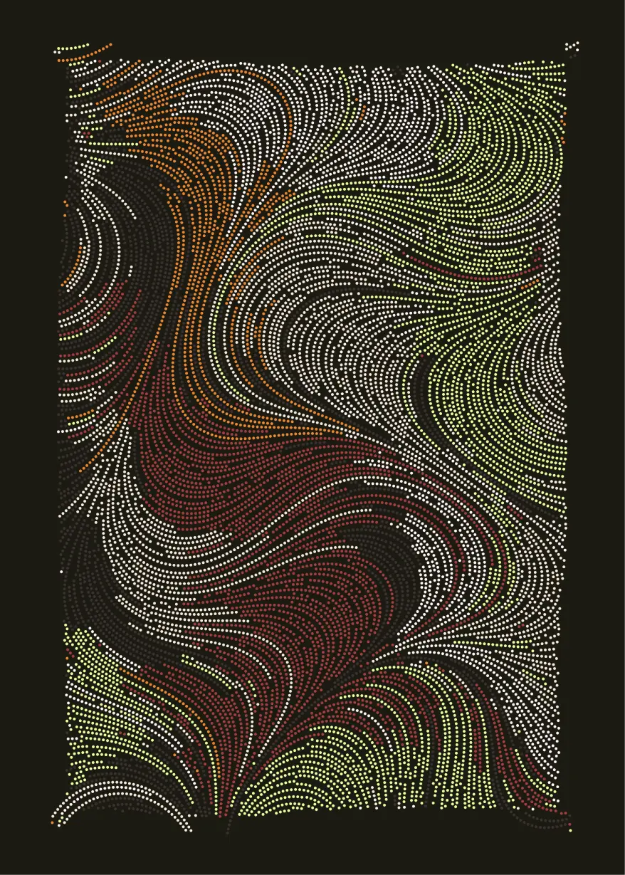
This article will describe the methods and concepts I used to create the series of generated artworks pictured below. I've tried to visualize the algorithms and provide some code samples. The code samples are written in a Typescript with some simplifications so that the code is readable on mobile and to make them more concise and easy to follow. The general algorithms can easily be ported to any language though, I have for instance done some implementations using Rust.

As a note, far more talented people than me have written articles on the subject upon which my work is very obviously based. I recommend reading that one too!

Noise functions

The main driving force behind these flow field images is usually a noise function. Without regurgitating the wikipedia article, a noise function is a function that takes a coordinate in 2d space (higher dimension noise-functions also exist, but are irrelevant for the purpose of this article) and returns a value in the range -1..=1 such as points close together return similar, but slightly different, values.

The interactive illustration below shows how this works by uniformly sampling points in a grid and calling the noise function for that point. Note that the values have been rounded to one decimal for legibility, the actual values have far more precision. Click Regenerate to run the noise function again with a new seed to get new noise values.

And here is the code that generated the image above, abbreviated for clarity.

[object Object]

To make it a bit easier to digest, we can visualize this in a more effective manner by translating the noise values into degrees and draw lines from a starting position and a few pixels following the degree of the noise value.

[object Object]

This doesn't look like much currently. It would appear that lines are fairly disjointed and go off in seemingly random directions. Not at all the smooth effect we're going for.

It turns out that noise functions are pretty sensitive. You'd think that the points(1.0, 1.0) and (1.0, 2.0) would produce somewhat similar noise values, following the rule that points in close proximity yield fairly similar noise values, but they're not close enough to each other.

To combat this we can force our points to be closer together by just dividing our x and y coordinates by some smoothness constant. For example, the distance between our two example points was previously 1.0 for the y-axis, and 0.0 for the x-axis, for a total distance of 1.0.

If we divide all our x and y values by the constant smoothness = 100 we'd end up with: p1 = (0.01, 0.01), p2 = (0.01, 0.02), making the distance only 0.01, but keeping the relation between the points the same.

const smoothness = 20;
const p1 = [1.0, 1.0];
const p2 = [1.0, 2.0];
distance(p1, p2) // returns 1.0;
distance(
  [p1.x / 20, p1.y / 20],
  [p2.x / 20, p2.y / 20],
)  // returns 0.0500
        

The only change we need to make to our code is the following:

[object Object]

You can think of it as shrinking our domain to better fit the noise values. Or zooming in on the noise function if that helps.

As we can see by dragging the smoothness value up, closer to 100 in this case, the lines start to smooth out and patterns start to emerge.

Drawing lines.

At this point we know how to navigate the flow field. Pick any point P, read the noise value n for that point and increment P.x by cos(n) and P.y by sin(n) as well as some extra pixels that represents the distance we want to travel in the direction of the field.

We did this in the previous examples by sampling points in a grid and and having a fixed line length. To approximate the effect illustrated in the images at the beginning of this article a bit better another implementation is necessary. First we need to pick a random point on the canvas and then ride the flow field until we get out of bounds.

[object Object]

Going from the above example to drawing an actual line should now be trivial. Start at any given point on the canvas an instantiate your line, move through the field just as before, but instead of drawing a new point at the given position add it to the points for the line. Stop the loop when the line has reached the end of the canvas and finally draw the line.

[object Object]

Mouse over the illustration below to create new lines from your mouse position.

Experimenting with lines.

So far not a lot of variance has been achieved. All results, no matter what the seed of the noise function is, will yield somewhat similar images. There are a few ways to combat this, one way is by warping the noise value a bit, resulting in lines exaggerating their turns, this is done by simply multiplying the noise value by some constant before applying the cos() and sin() functions.

[object Object]

Another way is by varying the length of the steps each line takes between each step as it progresses through the field. Shorter steps yield much smoother curves while longer steps will make the lines a lot more jagged.

[object Object]

Alternatives to noise functions

So far we've been using a noise function called OpenSimplex.

OpenSimplex noise is an n-dimensional gradient noise function that was developed in order to overcome the patent-related issues surrounding Simplex noise, while continuing to also avoid the visually-significant directional artifacts characteristic of Perlin noise.

As alluded to in the quote, there are few different noise functions. A proper noise function is a bit complicated and out of scope for this article, but nothing is stopping us from writing a function that returns similar values for a given coordinate, that part can be done pretty easily.

These home grown functions won't yield as random seeming results as a noise function but they will let us control the final output much more. They will also let us be much more creative in trying new things out now that we can draw lines that reliably follow a path.

An easy first test we can do is simply taking a coordinate and return it's distance to another point that we'll call the focalPoint, just to see what would happen. This function would satisfy the rule that points close together yield similar values, making our lines nice and smooth.

[object Object]

Mouse over the illustration below to set a new focal point

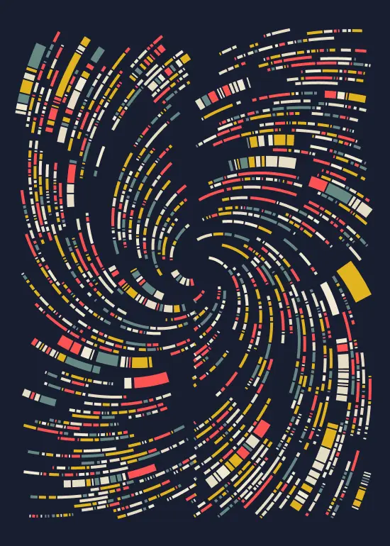
If we instead of returning the distance to focalPoint we can return the angle the line has from our point to and offset our point along the radius (with a slight distortion to the y-axis) we can get a nice swirl-like effect.

[object Object]

[object Object]

Collision Detection

In my opinion, the real fun doesn't really begin until we start looking at having the lines interact with each other. Instead of stopping when we reach the end of the canvas or we've reached the max line length we can instead stop when this line would collide with another line.

Hover the illustration (or slide your finger over it) to add lines of varying width.

Now, a lot can be said about collision detection and how to make it performant. I'll show only one method and a small optimization to keep the solution somewhat performant.

Checking the intersection of two straight lines isn't too bad and can be done in O(1) time. Our lines aren't straight however so we'll have to be a bit more clever. If we go back to the beginning of how we drew the line, it started with stepping through the noise field and adding a point for each step. If we made that point into a circle by giving it same radius as the line and kept track of each circle, not just in the line but in all lines it's a lot easier to check if the circle we are about to draw overlaps any other circle.

Checking if two circles overlap is only a matter of checking if the sum of their radii is smaller than the distance between their origo.

[object Object]

Here is another illustration that highlights when two non-linear lines meet using this method. Play with the illustration to move the colliding line.

[object Object]

Optimizing it slightly.

These example illustrations are fairly small so we haven't ran into any performance issues when checking if our line collides with any other line... yet. When trying to make a larger image however, in a print-friendly size for instance, we'd end up with a lot of lines with a lot of points that we could potentially collide with, meaning that for every new point we add we must check collisions against all other points. This stacks up fast and will make your render times a lot longer than desired. A way to mitigate this is to only check against points that are close enough for us to collide with.

The simplest way of doing that is by dividing our canvas up into a grid of boxes and whenever we are about to add a new point check which box it would go in, and then only check against collisions with points in that box.

Time for another illustration. This time, move your finger or mouse cursor around to see which points belong to the same box.

Now, with 100 boxes (10 across, 10 down) and if the points are distributed uniformly on the canvas, we end up doing 1/100^th as many checks that we did previously, increasing rendering performance by quite a bit! One thing to note however, is that if our boxes would be too small to reliably hold points with the radius of our lines then we'd start to get overlapping lines at the edges. This would also happen if a points origo was at the very edge of a box, causing its body to spill outside the boxes area. We could fix that by checking surrounding boxes for collisions as well, but that would mean we'd check another eight boxes besides the current one, increasing the search space a bit, but the result would be more exact.

A final optimisation we can do with this technique is that if our step size (the distance between each point in each line) is sufficiently small we could skip checking a few points in the box, since if our circle overlaps with one of the circles there's a high chance that it overlaps with some other circles as well. Now this might yield a less accurate result, but accuracy is not necessarly the end goal. Some small overlaps for a few lines might introduce some visually pleasing artifacts. Usually those kinds of details are happy little accidents.

[object Object]

Here we check against every 7^th circle in a box hoping to get a hit if there is one. The constant 7 might be too high in some cases, or could be increased even more, it all depends on the step size for the lines and can be tweaked to get a good balance between render times and correctness.

Finally, Colors.

The theme for this article is converging to "you can achieve a lot of variation with some tweaks". That's true for applying colors to these images as well. So far things in this article have been pretty monochrome to focus on the underlying techniques of how to achieve the overarching look.

The easiest way to get some color in there is to create a palette with a few different colors and picking at random when creating a new line.

[object Object]

Another coloring method is by coloring each line by the angle of the noise function where the line started. This will yield a gradient like coloring across larger images.

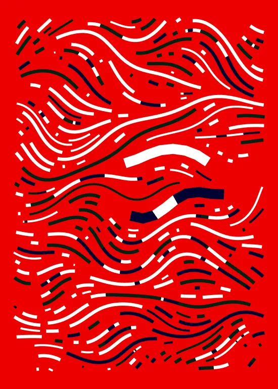
[object Object]

Finally, my favorite method is by subdividing the canvas into a set of regions, either by some Piet Mondrian Composition style, or recursively splitting the canvas into more and more refined polygons. After the canvas has been divided I assign each region a color and whenever a line spawns assign it the color of the region it spawned in.

This method creates a nice effect where things don't look as disjointed and more like streams of paint flowing into other buckets of paint.

Conclusion

Even though this article got quite long, it only scratches the surface of all the variants that can be achieved using the fundamental techniques described. I highly recommend trying things out and experimenting, swapping a cos() for a sin() somewhere, or maybe even a tan() if you're crazy.

Try subdividing the canvas into subregions who all have their own rules, or maybe dive deeper into noise functions. Or have a small border around the canvas and let some small percent of the lines escape it. Why use lines at all? Why not circles or squares or blobs?

Thanks for sticking in there this long, hope it was helpful.